Each experiment therefore consists of generating a time series of a particular length from the model, and applying HMMSeg (no smoothing) to the resulting time series, with nstates set to 2. The fitted parameters for emission and transition probabilities are then compared to those of the generative model. The accuracy of the state assignment (concordance) is also measured, by computing the percent of observations that were assigned by HMMSeg to the same state as that of the generative model.
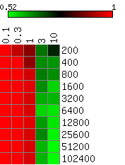
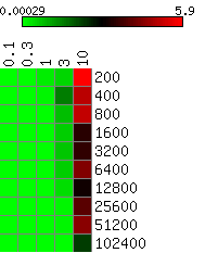
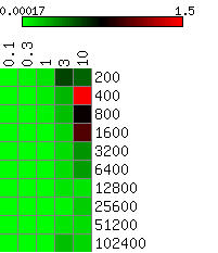
The heatmaps below show the average differences between the actual and the HMMSeg-predicted emission means and standard deviations, and the segmentation concordance. The standard deviation sigma was varied over the set 0.1, 0.3, 1, 3, and 10, and the time series length N varied from 200 to 102,400 (ten different lengths), for a total of 50 combinations of sigma and N. We performed 10 separate simulations for each (sigma, N) pair, for a total of 500 simulations. Each box in the heatmap reflects the average over ten simultaions. Column headers are emission standard deviations, and row headers are time series lengths. Heatmaps were generated using matrix2png.
We see that HMMSeg is generally very successful in recapitulating all of the generative model parameters and segmentations for sigma < = 1. Performance degrades rapidly for sigma > = 3. Although there seems to be improvement in all accuracy measures as N increases from 200 to 800, there is no clear further improvement when N increases past 800.
Larger values indicate greater degrees of agreement with the correct segmentation.
Smaller values indicate smaller differences (greater degrees of agreement) between the actual mean of 0 and the estimated mean.
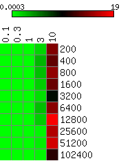
Smaller values indicate smaller differences (greater degrees of agreement) between the actual mean of 1 and the estimated mean.
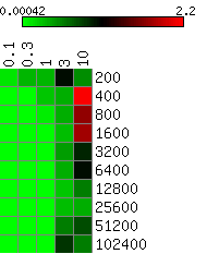
Smaller values indicate smaller differences (greater degrees of agreement) between the actual standard deviation indicated in the column header and the estimated standard deviation.
Smaller values indicate smaller differences (greater degrees of agreement) between the actual standard deviation indicated in the column header and the estimated standard deviation.
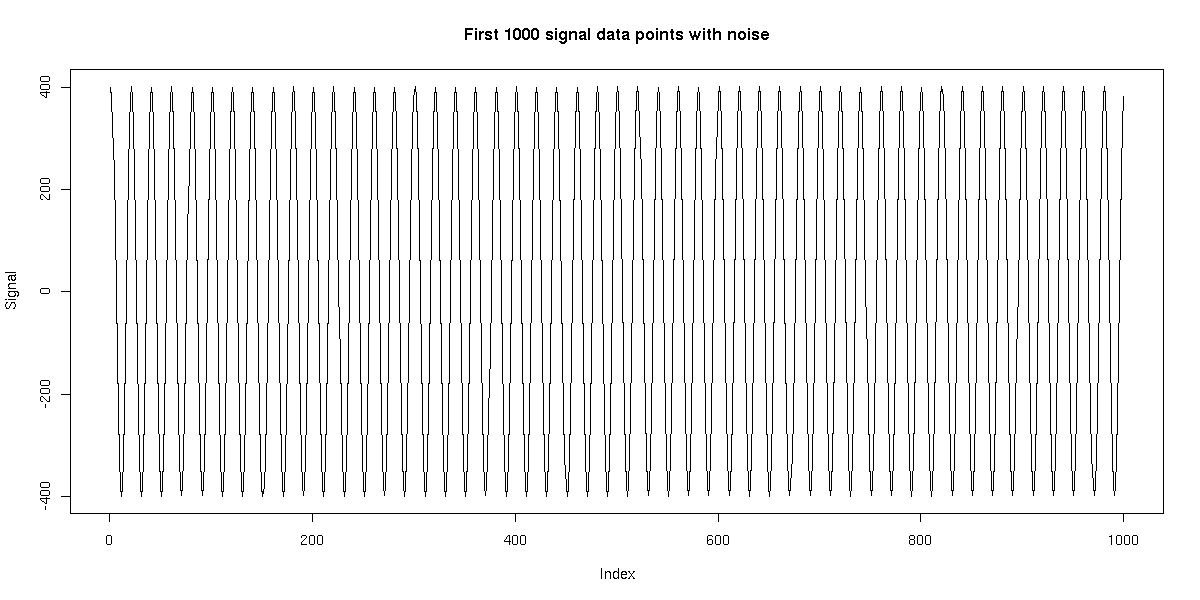
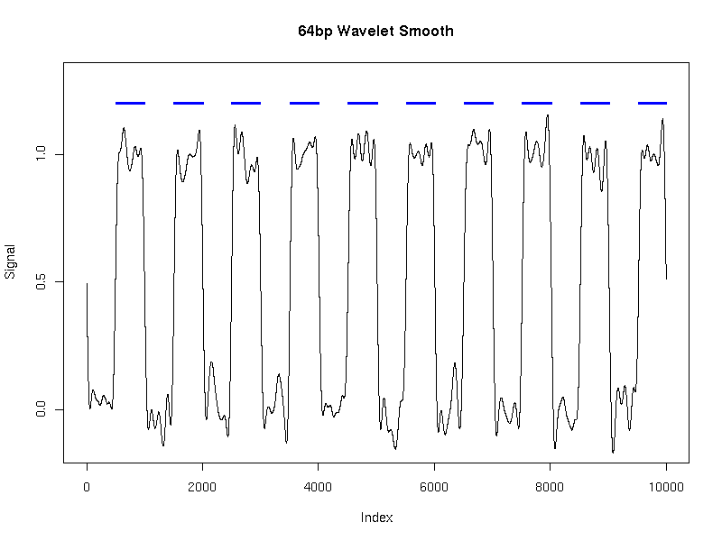
We generated a single time series of length 10,000 using this model. We then applied HMMSeg to the raw data, and to the 64bp wavelet-smoothed data. The chart below illustrates the futility of trying to recover the embedded signal without wavelet noise reduction - the concordance of the final segmentation with the original segmentation is 50%, or essentially no better than random. When wavelet smoothing is applied, however, the concordance jumps to 97%. The figures below illustrate the effect.
Time series: length 10000, resolution 1 bp, alternating length-500 segments
Noise on top of signal described below: 400 cos(pi * i / 10) (20-bp period)
Smoothing scale: 64 bp
| Statistic | Actual model | HMMSeg model (unsmoothed) | HMMSeg model (smoothed) |
|---|---|---|---|
| State 0 mean | 0 | -248.22 | 0.06 |
| State 0 standard deviation | 0.5 | 130.91 | 0.178 |
| State 0 state-switch probability | 0.002 | 0.099 | 0.002 |
| State 1 mean | 1 | 255.79 | 0.993 |
| State 1 standard deviation | 0.5 | 125.93 | 0.069 |
| State 1 state-switch probability | 0.002 | 0.101 | 0.002 |
| Percent agreement with actual segmentation | n/a | 50 | 97 |
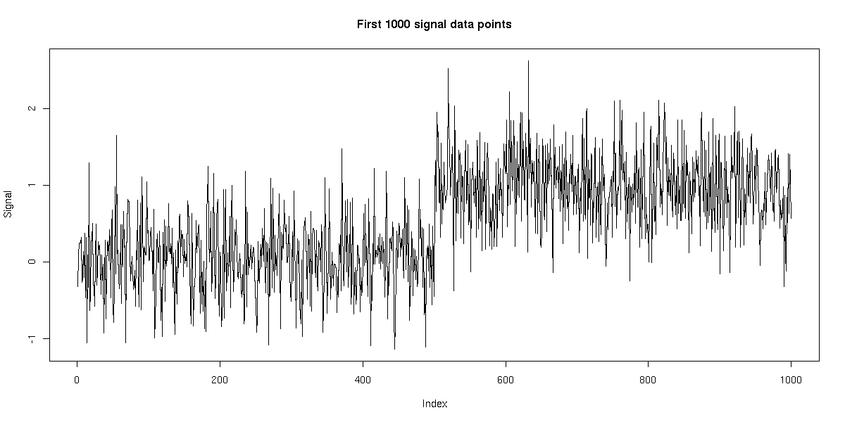
All plots below were generated using R.
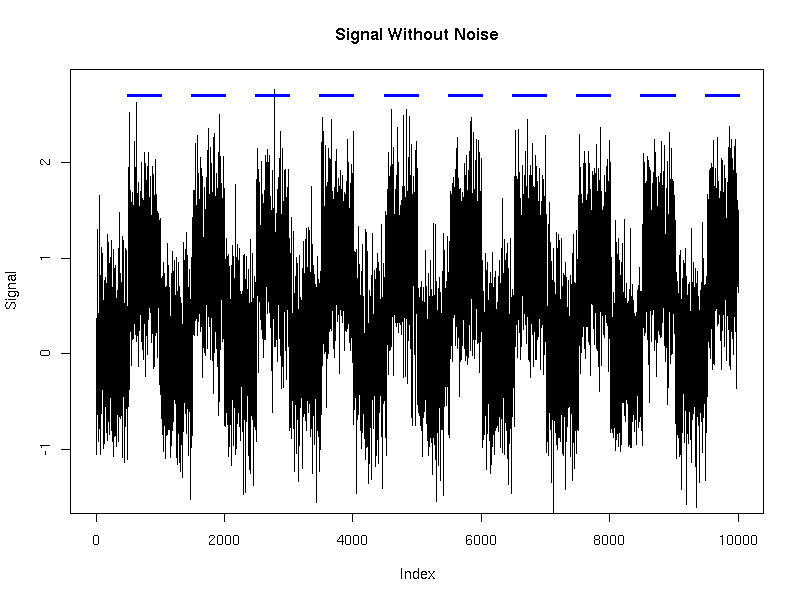
Without noise:
With noise: